Chapter 3.0 – The ML Project Workflow
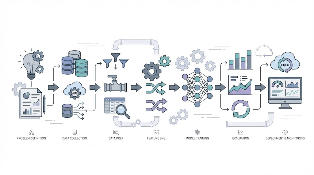
The complete end-to-end ML workflow mapped to automation concepts. From problem definition to production deployment.
Putting It All Together: From Scattered Concepts to Complete Workflow
Why this chapter?
If the last few chapters felt like puzzle pieces, this is where they come together. Here, you’ll see the full ML project workflow, how each step connects to what you’ve already learned, and how it sets you up for the advanced topics ahead.
Automation anology This is like learning individual Terraform/Ansible resources—important, but scattered. I needed to see the complete workflow from problem → production.
How to use this chapter:
This chapter is that workflow. It’s my attempt to document the end-to-end ML journey I wish I had when starting. Each phase links back to earlier chapters—revisit those if you need a refresher. This is your bridge from learning concepts to building real solutions.
Review: What You’ve Learned So Far
- Series 0: Why this matters for automation engineers (Chapter 0.1)
- Series 1: What AI is (1.1), how machines learn (1.2), ML types (1.3)
- Series 2: Data quality (2.1), features/labels (2.2), training vs inference (2.3)
Why This Structure Matters (Analogy)
Automation analogy:
- Series 0-2 = Learning what aws_instance, aws_vpc, variables, state files mean.
- Chapter 3.0 = Your first complete project: VPC → Subnet → EC2 → Deploy → Monitor.
- Series 3+ = Advanced patterns, modules, remote state, team workflows.
Confidence check: The phase mappings below connect to previous chapters. If something doesn’t make sense, it means either (a) I’m still learning that part, or (b) the reference is wrong—let me know!
1. The Seven Phases
Every ML journey follows this pattern:
flowchart TD
    Start([New ML Project])

    subgraph Phase1["📋 PHASE 1: DEFINE"]
        P1[Frame the Problem]
        P2[Select Performance Measure]
        P3[Check Assumptions]
        P1 --> P2 --> P3
    end

    subgraph Phase2["📊 PHASE 2: GET DATA"]
        D1[Create Workspace]
        D2[Download Data]
        D3[Quick Look at Structure]
        D4[Create Test Set]
        D1 --> D2 --> D3 --> D4
    end

    subgraph Phase3["🔍 PHASE 3: EXPLORE"]
        E1[Visualize Data]
        E2[Look for Correlations]
        E3[Experiment with Combinations]
        E1 --> E2 --> E3
    end

    subgraph Phase4["🔧 PHASE 4: PREPARE"]
        R1[Clean Data]
        R2[Handle Categories]
        R3[Custom Transformers]
        R4[Feature Scaling]
        R5[Build Pipeline]
        R1 --> R2 --> R3 --> R4 --> R5
    end

    subgraph Phase5["🔨 PHASE 5: TRAIN"]
        T1[Select Algorithm]
        T2[Train on Training Set]
        T3[Cross-Validation]
        T4[Fine-Tune Hyperparameters]
        T1 --> T2 --> T3 --> T4
    end

    subgraph Phase6["✅ PHASE 6: EVALUATE"]
        V1[Analyze Errors]
        V2[Test on Test Set]
        V3[Final Validation]
        V1 --> V2 --> V3
    end

    subgraph Phase7["⚡ PHASE 7: DEPLOY"]
        L1[Launch to Production]
        L2[Monitor Performance]
        L3[Maintain System]
        L4{Retrain?}
        L1 --> L2 --> L3 --> L4
    end

    Start --> Phase1
    Phase1 --> Phase2
    Phase2 --> Phase3
    Phase3 --> Phase4
    Phase4 --> Phase5
    Phase5 --> Phase6
    Phase6 --> Phase7
    L4 -->|Yes| Phase2
    L4 -->|No| L2

    style Phase1 fill:#e1f5ff,stroke:#0066cc,stroke-width:2px
    style Phase2 fill:#ffe1f5,stroke:#cc0066,stroke-width:2px
    style Phase3 fill:#fff3e1,stroke:#cc8800,stroke-width:2px
    style Phase4 fill:#e1ffe1,stroke:#00cc66,stroke-width:2px
    style Phase5 fill:#f0e1ff,stroke:#8800cc,stroke-width:2px
    style Phase6 fill:#ffe1e1,stroke:#cc0000,stroke-width:2px
    style Phase7 fill:#FFD700,stroke:#B8860B,stroke-width:3px
Automation analogy: It’s like your IaC workflow:
- Requirements → Design → Code → Test → Deploy → Monitor → Maintain.
2. The Detailed Steps
Here’s the complete checklist. Keep this handy when starting your ML journey.
Phase 1: Define the Problem
Why this connects: Remember Chapter 1.1 where we learned ML = pattern recognition in data? And Chapter 1.3 where we saw supervised vs unsupervised learning? This is where you decide which approach fits your problem.
| Step | What | Why |
|---|---|---|
| 1. Frame the problem | Define what you’re predicting and why ML helps | Is this supervised (predicting labels) or unsupervised (finding patterns)? See 1.3 |
| 2. Select metrics | Decide how to measure success (accuracy, precision, recall) | Like defining SLAs for your platform (Will cover in Chapter 3.3) |
| 3. Check assumptions | Verify you have data, features are available, problem is solvable | Do you have enough training examples? See 1.2 on learning from data |
Example: Deployment Risk Prediction
- Predict: High/Medium/Low risk before deployment
- Metrics: 90% precision (don’t block safe deployments), 85% recall (catch risky ones)
- Assumptions: ✅ 10K past deployments, ✅ Features available pre-deployment
Phase 2: Get the Data
Why this connects: Chapter 2.1 taught us garbage in = garbage out. Data quality matters MORE than fancy algorithms. Here’s where you apply that.
| Step | What | Why |
|---|---|---|
| 4. Create workspace | Set up project structure (data/, models/, notebooks/) | Like organizing Terraform modules and environments |
| 5. Download data | Pull from databases, APIs, logs | Like exporting current state |
| 6. Quick look | Check size, types, missing values, balance | Apply 2.1: completeness, accuracy, consistency |
| 7. Create test set | Set aside 20% for final evaluation, LOCK IT AWAY | Simulates future data—see 2.3 on validation vs test sets |
Critical: Never touch the test set until the very end. It simulates future production data.
Phase 3: Explore the Data
Why this connects: Chapter 2.2 explained features = the inputs ML uses to learn. Good features → better predictions. This phase finds those good features.
| Step | What | Why |
|---|---|---|
| 8. Visualize | Histograms, scatter plots, time series | Spot patterns and outliers |
| 9. Correlations | Which features relate to the outcome? | Find predictive signals—remember 2.2 on feature importance |
| 10. Feature combinations | Create new features by combining existing ones | Feature engineering from 2.2: risk_score = failures × changes |
Findings shape preparation:
- If
previous_failurescorrelates 0.78 with risk, keep it.- If
teamcorrelates 0.12, maybe drop it.
Phase 4: Prepare the Data
Foundation: Chapter 2.1 (Data Quality), Chapter 2.2 (Features & Labels)
For practical techniques and real-world tips on feature engineering, see Chapter 3.4 – Feature Engineering. (See mapping table above)
| Step | What | Why |
|---|---|---|
| 11. Clean data | Handle missing values (fill, drop, or indicate) | ML algorithms need complete data (Chapter 2.1) |
| 12. Encode categories | Convert text to numbers (one-hot, label encoding) | ML needs numeric inputs (Chapter 2.2) |
| 13. Custom transformers | Build reusable transformation components | Ensure same logic in training and production (Chapter 2.3) |
| 14. Feature scaling | Normalize ranges (0-1 or mean=0, std=1) | Prevent large values from dominating |
| 15. Build pipeline | Chain all transformations together | Reproducible and production-ready |
Pipeline example:
1
2
3
4
5
pipeline = Pipeline([
    ('imputer', SimpleImputer()),      # Fill missing values
    ('scaler', StandardScaler()),      # Normalize
    ('encoder', OneHotEncoder())       # Encode categories
])
Automation analogy: Like a CI/CD pipeline— same steps, same order, every time.
Phase 5: Train the Model
Why this connects: Chapter 1.2 showed us machines learn by adjusting parameters to minimize errors. Chapter 2.3 explained training = build time. Now we actually train.
For help choosing the right algorithm, see Chapter 3.1 – Common ML Algorithms. (See mapping table above)
| Step | What | Why |
|---|---|---|
| 16. Select algorithm | Decision Tree, Random Forest, etc. | Different algorithms for different problems (Will cover in Chapter 3.1) |
| 17. Train | Fit model on training data | The “learning” from 1.2—adjust weights to minimize error |
| 18. Cross-validate | Test on 5 different splits | The validation strategy from 2.3—prevents overfitting |
| 19. Fine-tune | Grid/random search for best hyperparameters | Hyperparameter tuning from 2.3—optimize learning |
Quick start: Begin with Decision Tree or Random Forest. They work well out-of-the-box.
Phase 6: Evaluate
Foundation: Chapter 2.3 (Training vs Inference)
For understanding overfitting/underfitting, see Chapter 3.2 – Overfitting & Underfitting.
For evaluation metrics and honest model assessment, see Chapter 3.3 – Model Evaluation. (See mapping table above)
| Step | What | Why |
|---|---|---|
| 20. Analyze errors | Where does the model fail? | Identify improvement opportunities (Will cover in Chapter 3.2) |
| 21. Test set evaluation | NOW test on locked-away test set (once!) | Honest estimate of production performance (Chapter 2.3) |
Expected: Test score should be within 2-3% of cross-validation score. If much worse, you overfit.
Phase 7: Deploy and Monitor
Foundation: Chapter 2.3 (Inference & Retraining)
| Step | What | Why |
|---|---|---|
| 22. Launch | Save model, version it, deploy to production | Make predictions available (Chapter 2.3) |
| 23. Monitor | Track accuracy, latency, prediction distribution | Catch degradation early (Chapter 2.3) |
| 24. Maintain | Retrain when accuracy drops or data drifts | Keep model relevant (Chapter 2.3) |
Monitoring triggers:
- Accuracy < 85%? Retrain.
- 30 days since last train? Retrain.
- Data patterns changed? Retrain.
Automation analogy: Like GitOps—deploy, monitor CloudWatch/Datadog, update based on metrics.
3. Quick Reference Checklist
Key Takeaways:
- ML projects follow a repeatable workflow, just like automation projects.
- Data quality and preparation matter more than fancy algorithms.
- Never touch your test set until the very end.
- Monitor and retrain models as you would update and monitor infrastructure.
Print this and check off as you go:
Define
- Frame problem
- Select metrics
- Verify assumptions
Get Data
- Create workspace
- Download data
- Quick structure review
- Create & lock test set
Explore
- Visualize distributions
- Calculate correlations
- Engineer feature combinations
Prepare
- Clean (missing values)
- Encode categories
- Scale features
- Build pipeline
Train
- Select algorithm (3.1)
- Train on training set
- Cross-validate
- Fine-tune hyperparameters
Evaluate
Deploy
- Launch to production
- Set up monitoring
- Schedule retraining
4. What’s Next
Architectural Question: How do the phases of an ML project map to automation workflows, and what are the key checkpoints for success?
The chapters ahead dive into specific steps:
- Chapter 3.1: Common algorithms (when to use Decision Trees vs Random Forest vs others)
- Chapter 3.2: Overfitting/underfitting (why models fail in prod)
- Chapter 3.3: Evaluation metrics (accuracy, precision, recall explained)
This workflow is your map. The upcoming chapters explore the terrain.