Chapter 2.1 – Data: The New Configuration File

---

When Bad Data Breaks Everything

---

After learning about ML types, I realized: Bad data doesn’t just break systems—it teaches models to make wrong predictions.

What if the historical deployment data is incomplete or wrong?

In automation, bad config or variables cause immediate failures. In ML, bad data can silently lead to confident, wrong predictions.

Warning: Bad data = bad model. No matter how sophisticated the algorithm, if the training data is garbage, the predictions will be garbage.

What I’m documenting here:

• My evolving understanding of data quality
• Why it matters more than I thought
• How to prepare data for ML (from an automation mindset)

---

1. What I Learned About Data Requirements

At first, I thought: “I have deployment logs, so I have data. Done.” Not quite.

The real issues are:

• Quality: Does the data represent the problem?
• Quantity: Is there enough to learn patterns?
• Balance: Is it biased toward one outcome?
• Relevance: Do the features actually predict what matters?

My realization: Having data ≠ having the right data.

In automation, wrong variables break infra. In ML, wrong data breaks predictions—often silently.

What I Learned About Data vs Algorithms

One paper changed my thinking: In 2009, Google researchers (including Peter Norvig) showed that for many complex problems, more data with simpler algorithms often beats less data with sophisticated algorithms.

Key insight: “Choose a representation that can use unsupervised learning on unlabeled data, which is so much more plentiful than labeled data.”

Focus on quality and quantity of data before worrying about the perfect algorithm.

---

2. Data: The New Configuration File

For Automation Engineers

When you write Terraform or Ansible, you work with:

See Example: Terraform Variables

# Terraform variables
variable "instance_type" {
  type    = string
  default = "t3.medium"
}

variable "environment" {
  type    = string
  validation {
    condition     = contains(["dev", "staging", "prod"], var.environment)
    error_message = "Invalid environment"
  }
}

These variables define the inputs to your automation logic.

For Machine Learning

In ML, data serves the same purpose:

See Table: Automation vs ML Concepts

Automation Concept	ML Equivalent	Purpose
Configuration file	Training dataset	Defines what the system should learn
Variable validation	Data quality checks	Ensures inputs are valid
State file	Model weights	Captures learned patterns
Outputs	Predictions	What the system produces

Tip: Just as you validate Terraform variables, you must validate training data.

---

3. The “Garbage In, Garbage Out” Principle I Learned

Why ML Is Scarier Than Automation

In automation, if I run:

terraform apply -var="instance_type=invalid_type"

Result: Immediate failure with a clear error message.

I fix the variable and try again. Fast feedback loop.

---

What I Learned About ML

Now imagine training an ML model with:

• Mislabeled data
• Missing values
• Biased samples
• Inconsistent formats

Result: Model succeeds in training (no errors)

But: Model fails in production (wrong predictions)

This is what scared me:

• Bad data doesn’t cause training to fail
• It causes the model to confidently learn the wrong patterns

Example That Made It Real

Thinking about deployment risk assessment:

Goal: Predict deployment risk (High/Medium/Low)

What if the training data has problems?

See Table: Data Issues and Model Impact

Data Issue	What The Model Learns
All “High risk” deployments mislabeled as “Low risk”	Model learns backwards—predicts safe when dangerous
Missing “time of day” for night deployments	Model never learns that 3 AM deployments are riskier
Only includes successful deployments	Model can’t recognize failure patterns
Biased toward one team’s deployments	Model performs poorly for other teams

Each issue creates a model that appears to work in training but makes dangerous predictions in production.

Warning: The silent failure to watch for—bad data can make your model appear to work in training but make dangerous predictions in production.

---

4. Data Quality Checklist I’m Using

Before training any model, I now ask:

1. Completeness

Is all required data present?

# Automation mindset
required_vars = ["instance_type", "vpc_id", "subnet_id"]
missing = [v for v in required_vars if v not in config]

# ML mindset
required_features = ["deployment_size", "time_of_day", "change_count"]
missing = df[required_features].isnull().sum()

For deployment risk:

• Do all deployments have timestamp?
• Do all have team information?
• Do all have outcome (success/failure)?

2. Accuracy

Is the data correct?

• Automation: Instance type “t3.mediam” (typo) → deployment fails immediately
• ML: Deployment labeled “High risk” but actually succeeded → model learns wrong pattern

For deployment risk:

• Are risk labels verified?
• Are timestamps in correct timezone?
• Are failure reasons accurately recorded?

3. Consistency

Is the data formatted uniformly?

See Table: Data Consistency Issues

Inconsistent Data	Problem
Team names: “DevOps”, “devops”, “Dev-Ops”	Model treats as 3 different teams
Timestamps: UTC vs local time	Time-based patterns break
Risk levels: “HIGH” vs “high” vs “H”	Labels don’t match

Best Practice: Normalize your data before training, just like normalizing Terraform variable names.

4. Relevance

Does the data actually predict what you care about?

• Automation: Checking instance color doesn’t tell you if deployment will succeed
• ML: Developer’s favorite coffee ☕ doesn’t predict deployment risk

For deployment risk:

• Include: deployment size, time, change count, environment
• Exclude: developer name, commit message length, office location

5. Timeliness

Is the data recent and representative?

• Problem: Training on 2-year-old deployment data
• Reality: Your infrastructure, processes, and teams have changed

Best Practice: Use recent data and retrain periodically (we’ll cover this in the MLOps series).

6. Representativeness

Does the training data represent the real-world cases you’ll encounter?

Key principle: In order to generalize well, your training data must be representative of the new cases you want to predict.

Automation example:
Testing deployments only during business hours
Reality: Production deployments happen 24/7, including weekends

ML example:
Training deployment risk model only on small deployments (< 50 files)
Reality: Production includes large deployments (500+ files)

For deployment risk:

See Table: Representativeness Issues

Training Data	Real World	Problem
Only weekday deployments	Weekend deployments happen	Model has never seen weekend patterns
Only one cloud region	Multi-region deployments	Different regions have different behaviors
Only successful deployments	Need to predict failures	Model can’t recognize failure patterns
Only Team A’s deployments	All teams deploy	Model biased toward Team A’s practices

Solution: Ensure training data covers:

• All time periods (weekday, weekend, day, night)
• All environments (dev, staging, prod)
• All teams and regions
• Both successes AND failures
• Full range of deployment sizes

Tip: Representativeness is about coverage of real-world scenarios. Even unbiased data can be non-representative if it doesn’t cover the variety of cases you’ll see in production.

---

5. Data Preparation: The Pipeline

Just as you have CI/CD pipelines for code, you need data pipelines for ML.

flowchart LR
  A[Raw Data] --> B[Cleaning]
  B --> C[Validation]
  C --> D[Transformation]
  D --> E[Feature Engineering]
  E --> F[Ready for Training]
    
  style A fill:#e1f5ff
  style B fill:#ffe1e1
  style C fill:#fff4e1
  style D fill:#e1ffe1
  style E fill:#f0e1ff
  style F fill:#90EE90

Step 1: Cleaning

Remove or fix problematic data:

See Example: Data Cleaning (Python)

# Remove duplicates
df = df.drop_duplicates()

# Handle missing values
df['deployment_size'].fillna(df['deployment_size'].median(), inplace=True)

# Remove outliers (deployments > 10,000 files likely errors)
df = df[df['files_changed'] < 10000]

Automation Parallel: Removing invalid configuration entries is like cleaning your ML data.

Step 2: Validation

Ensure data meets quality standards:

See Example: Data Validation (Python)

# Check for required fields
assert df['timestamp'].notnull().all(), "Missing timestamps"

# Validate ranges
assert (df['risk_level'].isin(['High', 'Medium', 'Low'])).all()

# Check distribution (avoid extreme bias)
print(df['risk_level'].value_counts())

Automation Parallel: terraform validate before apply is like validating your ML data before training.

Step 3: Transformation

Convert data to usable formats:

See Example: Data Transformation (Python)

# Convert timestamps to features
df['hour'] = df['timestamp'].dt.hour
df['day_of_week'] = df['timestamp'].dt.dayofweek
df['is_weekend'] = df['day_of_week'].isin([5, 6])

# Encode categorical variables
df['environment_encoded'] = df['environment'].map({
  'dev': 0, 'staging': 1, 'prod': 2
})

Automation Parallel: Converting YAML to JSON for API consumption is like transforming your ML data into usable formats.

Step 4: Feature Engineering

Create new features from existing data (we’ll dive deeper into this in a moment):

See Example: Feature Engineering (Python)

# Create composite features
df['deployment_velocity'] = df['files_changed'] / df['deployment_duration']
df['risk_score'] = df['files_changed'] * df['is_prod'] * df['is_weekend']

Automation Parallel: Creating derived Terraform locals from variables is like feature engineering in ML.

---

6. Feature Engineering: Creating Better Inputs

Feature engineering is the process of transforming raw data into features (inputs) that better represent the problem.

Why It Matters

Going back to our Terraform analogy:

See Example: Feature Engineering Analogy (Terraform)

# Raw inputs
variable "instance_count" { default = 5 }
variable "instance_type" { default = "t3.medium" }

# Derived values (locals)
locals {
  total_vcpus = var.instance_count * lookup(local.instance_vcpu_map, var.instance_type)
  estimated_cost = local.total_vcpus * var.hourly_rate
}

The estimated_cost is more useful for decision-making than raw inputs.

ML Feature Engineering Example

Raw features:

• files_changed: 150
• hour: 14
• day_of_week: 2

Engineered features:

• deployment_size_category: “Large” (if > 100 files)
• is_business_hours: True (if 9 AM - 5 PM)
• is_risky_time: False (if weekend OR after-hours)

The engineered features make patterns easier for the model to learn.

For Deployment Risk Assessment

See Table: Raw vs Engineered Features

Raw Data	Engineered Feature	Why It Helps
files_changed: 200	is_large_deployment: True	Simplifies threshold learning
timestamp: 2026-01-07 03:00	is_late_night: True	Captures risk pattern directly
previous_failures: [3, 0, 1, 2]	failure_rate: 0.25	Aggregates history
team: "Platform"	team_experience_score: 0.9	Incorporates team reliability

Engineering Insight: Help the model by giving it features that directly relate to the problem.

---

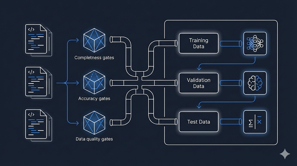
7. Data Splits: Training, Validation, and Test

When you develop automation code, you test in multiple environments:

Dev → Staging → Production

In ML, you split your data into three sets:

Training → Validation → Test

The Three Splits Explained

flowchart TB
    A[All Available Data] --> B[Training Set<br/>60-70%]
    A --> C[Validation Set<br/>15-20%]
    A --> D[Test Set<br/>15-20%]
    
    B --> E[Model Learns<br/>from This]
    C --> F[Tune & Adjust<br/>Using This]
    D --> G[Final Evaluation<br/>Never Seen Before]
    
    style A fill:#e1f5ff
    style B fill:#90EE90
    style C fill:#fff4e1
    style D fill:#ffe1e1
    style E fill:#e1ffe1
    style F fill:#fff4e1
    style G fill:#ffcccc

Training Set (60-70%)

Purpose: The data the model learns from

• Automation analogy: Your dev environment where you experiment and iterate
• For deployment risk: Use 70% of historical deployments to train the model on patterns

Validation Set (15-20%)

Purpose: Tune the model and check performance during development

• Automation analogy: Staging environment where you verify before production
• For deployment risk: Use 15% of deployments to validate the model isn’t overfitting (we’ll cover this in Chapter 3.2)

Important: You can look at validation results and adjust your model based on them

Test Set (15-20%)

Purpose: Final evaluation on completely unseen data

• Automation analogy: Production deployment—the real test
• For deployment risk: Use 15% of deployments as a final check before deploying the model

Best Practice: Never look at test data during development. Only use it once at the very end.

Why This Matters

Bad practice:

# Train on ALL data
model.fit(all_data)

# Test on same data
accuracy = model.score(all_data)  # 99% accurate! 🎉

Warning: If you train and test on the same data, the model memorizes instead of learning patterns—leading to failure on new deployments.

Good practice:

# Split data
train, val, test = split_data(all_data, [0.7, 0.15, 0.15])

# Train on training set
model.fit(train)

# Tune using validation set
model.adjust_based_on(val)

# Final test on unseen data
final_accuracy = model.score(test)  # 85% (realistic)

---

8. Data Bias: The Hidden Danger

Bias in data is like bias in configuration—it leads to inconsistent and unfair outcomes.

Types of Bias

1. Sample Bias

Definition: Your training data doesn’t represent reality

• Automation: Testing only on t3.medium instances, then deploying to t3.large—things break
• ML: Training deployment risk model only on Platform team’s deployments
  • Result: Model performs poorly for other teams

2. Historical Bias

Definition: Past decisions were biased, and model learns those biases

• Example:
  • Historical data: “All deployments by Team X flagged as High Risk”
  • Reason: Team X was new and had early failures
  • Model learns: “Team X = High Risk” even though team improved

Best Practice: Use recent data and weight recent examples more heavily to avoid historical bias.

3. Measurement Bias

Definition: How you measure/label data introduces bias

• Example:
  • “High risk” defined by one person’s judgment
  • Different people have different risk tolerance
  • Model learns inconsistent labels

Best Practice: Standardize your labeling process and use objective criteria to avoid measurement bias.

Detecting Bias

Check your data distribution:

# Check distribution across teams
print(df.groupby('team')['risk_level'].value_counts())

# Output might show:
# Team A: 80% Low Risk, 15% Medium, 5% High
# Team B: 30% Low Risk, 30% Medium, 40% High  ← Biased!

Tip: If one group is disproportionately labeled as risky, investigate why—this may reveal hidden bias in your data.

---

9. Practical Guidelines for Data Preparation

Based on automation engineering principles:

1. Automate Data Validation

Automate checks to ensure your data meets quality standards before training.

Best Practice: Automate data validation to catch issues early, just like you would with infrastructure code.

See Example: Automate Data Validation

def validate_deployment_data(df):
  """
  Validate deployment data quality
  Like 'terraform validate' but for ML data
  """
  checks = {
    'no_missing_timestamps': df['timestamp'].notnull().all(),
    'valid_risk_levels': df['risk_level'].isin(['High', 'Medium', 'Low']).all(),
    'reasonable_file_counts': (df['files_changed'] > 0).all() & (df['files_changed'] < 10000).all(),
    'recent_data': (df['timestamp'] > '2024-01-01').all()
  }
    
  failed = [k for k, v in checks.items() if not v]
  if failed:
    raise ValueError(f"Data validation failed: {failed}")
    
  return True

2. Version Your Data

Keep track of changes in your data just like you version your code or infrastructure.

See Example: Version Your Data

data/
  ├── v1.0/
  │   └── deployment_history.csv
  ├── v1.1/
  │   └── deployment_history.csv  # Added new features
  └── v2.0/
      └── deployment_history.csv  # Changed labeling criteria

Best Practice: Track what changed between data versions (we’ll cover this more in the MLOps series).

3. Document Data Provenance

Document where your data comes from and any known issues for future reference.

Best Practice: Create a data README to document data provenance and known issues.

See Example: Data README (Provenance)

# Deployment Risk Dataset v2.0

## Source
- Extracted from: JIRA, Jenkins, GitLab
- Date range: 2024-01-01 to 2026-01-07
- Total deployments: 5,432

## Features
- `deployment_id`: Unique identifier
- `timestamp`: Deployment start time (UTC)
- `files_changed`: Number of files modified
- `risk_level`: High/Medium/Low (labeled by SRE team)

## Known Issues
- Missing data for deployments before 2024-01-01
- Team names not standardized until v2.0

## Last Updated
2026-01-07

4. Monitor Data Quality Over Time

Regularly check if your new data still matches the patterns and quality of your training data.

Best Practice: Continuously monitor for data drift to ensure your models remain reliable as new data arrives.

See Example: Monitor Data Quality Over Time

def monitor_data_drift(current_data, reference_data):
  """
  Check if new data distribution matches training data
  Like monitoring drift in Terraform state
  """
  metrics = {
    'avg_files_changed': current_data['files_changed'].mean(),
    'risk_distribution': current_data['risk_level'].value_counts(),
    'deployment_frequency': len(current_data) / days_span
  }
    
  # Compare with reference
  # Alert if significant drift detected

---

What I Wish I Knew Earlier

Practitioner’s Lessons:

• Data is configuration for ML: Bad data = bad model, just like bad variables = broken infrastructure.
• Quality matters more than quantity: 1,000 high-quality labeled deployments > 10,000 messy ones.
• Data preparation is not optional: It’s the foundation—skip it and your model will fail.
• Use train/validation/test splits: Like dev/staging/prod environments for code.
• Feature engineering amplifies signal: Help your model by creating meaningful features.
• Watch for bias: Biased data leads to biased models.
• Automate and version everything: Treat data pipeline like infrastructure code.

---

What’s Next?

➡ Series 2 – Chapter 2.2: Features, Labels, and Models

In the next chapter, we’ll explore:

• Features, labels, and models in detail
• How to choose the right features
• The relationship between inputs, logic, and outputs
• Building our first conceptual model for deployment risk

Architectural Question: How do you decide which features and labels are most important for building a reliable machine learning model in automation scenarios?

We’ve prepared the data—now we’ll use it to build something that learns.

---