Chapter 2.2 – Features, Labels, and Models

---

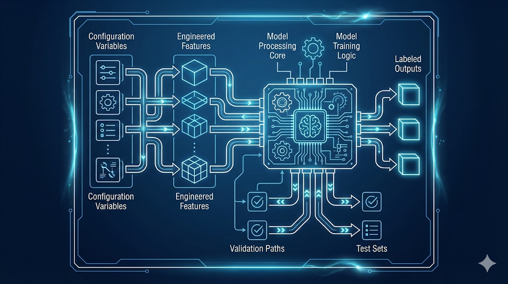
Decoding the ML Language: Inputs, Logic, and Outputs

---

After learning about data quality, I wondered: What does a model actually look at, and what is it trying to predict?

Turns out, ML uses the same pattern as automation—Inputs → Logic → Outputs.

• Features = Inputs (data the model sees)
• Model = Logic (learned, not hand-coded)
• Labels = Outputs (what you want to predict)

Key insight: These aren’t new concepts—just new names for a familiar pattern. In ML, the model learns the logic from examples, instead of you writing it.

---

1. Why Understanding This Helps

Every ML system—spam filter or ChatGPT—breaks down into:

• Features: What info does the system have?
• Labels: What is it trying to predict?
• Model: What logic connects them?

Once you see this, ML problems become easier:

• Start with “What am I predicting?” (labels)
• Then, “What inputs help predict it?” (features)
• Clear labels = clear success criteria

Automation analogy: Like knowing variables, logic, and outputs in code. You can’t build good infrastructure without knowing what inputs drive what outputs.

---

2. The Fundamental Pattern: Inputs → Logic → Outputs

Here’s how the Inputs → Logic → Outputs pattern looks in both automation and machine learning:

Automation (Terraform)

• Inputs: variables (instance_type, environment, instance_count)
• Logic: your code (resource definitions, rules)
• Outputs: what gets created (infrastructure, computed values)

See Automation Example (Terraform)

# Inputs (variables)
variable "instance_type" { default = "t3.medium" }
variable "environment" { default = "prod" }
variable "instance_count" { default = 3 }

# Logic (your code)
resource "aws_instance" "server" {
  count         = var.instance_count
  instance_type = var.instance_type
  tags = {
    Environment = var.environment
    CostCenter  = var.environment == "prod" ? "production" : "development"
  }
}

# Outputs (what gets created)
output "server_ips" {
  value = aws_instance.server[*].private_ip
}

Machine Learning

• Features: inputs (files_changed, environment, time_of_day, team)
• Model: learned logic (patterns from data)
• Label: output (e.g., “High Risk”)

See Machine Learning Example

# Features (inputs)
features = {
  'files_changed': 150,
  'environment': 'prod',
  'time_of_day': 14,
  'team': 'Platform'
}

# Model (learned logic)
model = trained_deployment_risk_model

# Label (predicted output)
prediction = model.predict(features)
# Output: **"High Risk"**

Engineering insight: In automation, you write the logic. In ML, the model learns the logic from examples.

No matter the domain, the core pattern is the same: you start with inputs, apply logic (written or learned), and get outputs.

---

3. Features: The Inputs to Your Model

What is a Feature?

A feature is a measurable property you feed into a model—think Terraform variables, but for ML.

Feature Types

• Numeric: quantifiable values (e.g., file count, time)
• Categorical: categories (e.g., environment, team)
• Boolean: true/false flags (e.g., is_weekend)

See deployment risk feature examples

Feature Name	Type	Example Value	What It Represents
files_changed	Numeric	150	Size of deployment
environment	Categorical	“prod”	Where deploying
time_of_day	Numeric	14 (2 PM)	When deploying
day_of_week	Numeric	2 (Tuesday)	Day of deployment
team	Categorical	“Platform”	Who is deploying
previous_failures	Numeric	3	Historical failures
deployment_duration_avg	Numeric	12.5 (minutes)	Team’s avg speed

Each feature is something the model can use to make predictions.

Good Features vs Bad Features

The best features are measurable, available before prediction, and make logical sense for the outcome.

See table: Good Features vs Bad Features

Feature	Type	Predictive Power	Why/Why Not?
files_changed	Numeric	✅ High	Large deployments are riskier
environment	Categorical	✅ High	Prod deployments need more care
previous_failures	Numeric	✅ High	History predicts future risk
developer_shirt_color	Categorical	❌ None	No relationship to deployment risk
commit_message_length	Numeric	❌ Low	Doesn’t indicate actual risk

Focus on features that are relevant, reliable, and available before prediction.

Automation Analogy: Just as you only use variables in Terraform that actually affect your infrastructure, in ML you want features that truly impact the outcome—not just any data you can collect.

See Quick Checklist: Picking the Right Features

| Principle | Good Example | Bad Example | | ----------------------------- | ----------------------------------------------- | ----------------------------------------------------------- | | Available at prediction time? | `files_changed` (known before deploying) | `deployment_outcome` (this is what we're predicting!) | | Correlated with the outcome? | `time_of_day` (night deployments are riskier) | `developer_coffee_preference` (tempting, but no) | | Reliable and consistent? | `environment` (always known) | `server_mood` (doesn't exist) | | Avoids leakage? | `historical_error_rate` (from past deployments) | `post_deployment_error_count` (only known after deployment) |

If your features pass these checks, you’re on the right track.

Warning: Data leakage is when you accidentally include information that wouldn’t be available in production. It’s like using terraform state as an input to terraform plan—you’re basically cheating by looking at the answer. Your model will look amazing in testing and fail miserably in production.

---

4. Labels: The Outputs You’re Predicting

Your model is only as good as your labels. Labels are the answers you want your model to predict.

What is a Label?

• The value you want to predict (e.g., “High Risk”).
• In automation, this is like a Terraform output.

See real-world label examples

Scenario	Features (Inputs)	Label (Output)
Email spam detection	Email text, sender, links	“Spam” / “Not Spam”
Image classification	Pixel values	“Cat” / “Dog” / “Bird”
Deployment risk	Files changed, time, team	“High” / “Medium” / “Low”
Server failure prediction	CPU, memory, disk usage	“Will fail” / “Won’t fail”

Label Types (Classification vs Regression)

This section and table compare the two main types of labels in machine learning: classification (categories) and regression (numeric values).

Label Type	What it Predicts	Example Label(s)	Example Use Case
Classification	Category/class	“High Risk”, “Low Risk”	Deployment risk
Regression	Numeric value	23.5 (minutes)	Deployment duration

Automation Analogy: Labels are like Terraform outputs—classification is like conditional outputs, regression is like numeric outputs.

Good vs Bad Labels: Quick Checklist

| Principle | Good Example | Bad Example | | --------------------- | ---------------------------------------------- | ---------------------------------------------- | | Clear & Unambiguous | deployment_succeeded: True/False | deployment_quality: Good/Bad | | Consistently Defined | All "High Risk" deployments meet same criteria | Different people label "High Risk" differently | | Verifiable | deployment_failed: True (check the logs) | deployment_felt_risky: True (opinion) | | Balanced Distribution | 40% Low, 35% Medium, 25% High | 95% Low, 4% Medium, 1% High |

Warning: Bad labels = bad model, just like bad configuration = broken infrastructure.

---

5. Models: The Learned Logic

What Is a Model?

A model is the learned logic that connects features (inputs) to labels (outputs). Instead of you writing the rules, the model discovers patterns by analyzing examples.

Automation Analogy: Like a Terraform config that transforms variables into outputs, but the logic is learned from data, not hand-coded.

The Mental Model

flowchart LR
  subgraph INPUTS["Features (Inputs)"]
    F1["files_changed = 150"]
    F2["environment = prod"]
    F3["team = platform"]
    F4["time_of_day = 14"]
    style F1 fill:#e1f5ff,stroke:#007acc,stroke-width:2px
    style F2 fill:#e1f5ff,stroke:#007acc,stroke-width:2px
    style F3 fill:#e1f5ff,stroke:#007acc,stroke-width:2px
    style F4 fill:#e1f5ff,stroke:#007acc,stroke-width:2px
  end

  INPUTS --> M["ML Model\n(Learned patterns from history)"]
  style M fill:#fff4e1,stroke:#ff9900,stroke-width:2px
  M --> L["Prediction\nHigh Risk Deployment"]
  style L fill:#d4f7d4,stroke:#228B22,stroke-width:2px

The model learns rules like:

IF files_changed > 100 AND environment == "prod" THEN risk = "High"
IF files_changed < 50 AND environment == "dev" THEN risk = "Low"
IF time_of_day BETWEEN 0 AND 6 THEN increase risk by one level

You don’t write these rules—the model finds them from data.

Models as Functions

Mathematically, a model is a function:

# Automation: You write the function
def calculate_cost(instance_count, instance_type, hours):
    hourly_rate = get_rate(instance_type)
    return instance_count * hourly_rate * hours

# ML: The model IS the function (learned from data)
def predict_risk(features):
    # Complex learned logic inside
    return risk_level  # "High" / "Medium" / "Low"

Terraform analogy:

# Your explicit logic
locals {
  is_production = var.environment == "prod"
  requires_approval = local.is_production && var.change_size > 100
}

# ML learned logic (conceptual)
model_logic {
  learned_pattern_1 = features.environment == "prod" && features.files_changed > 100
  learned_pattern_2 = features.previous_failures > 3
  learned_pattern_3 = features.time_of_day < 6 || features.time_of_day > 22
  risk = combine(learned_pattern_1, learned_pattern_2, learned_pattern_3)
}

What’s Inside a Model?

Every model type represents learned logic differently. Here’s how some common models work under the hood:

See table: Common Model Types & Automation Analogies

Model Type	Internal Logic	Automation Analogy
Decision Tree	Series of if-then rules	Nested Terraform conditionals
Linear Model	Weighted sum of features	Terraform locals with arithmetic
Neural Network	Layers of transformations	Pipeline of processing steps
Random Forest	Multiple decision trees voting	Multiple validation checks

Tip: For most use cases, treat the model as a black box that learned logic from data. You don’t need to understand the internals to use it effectively.

Model Artifacts

After training, a model becomes a set of files you can deploy:

See example: Model Artifacts

deployment-risk-model/
├── model.pkl                 # The learned weights/parameters
├── feature_names.json        # Which features it expects
├── label_mapping.json        # How it encodes outputs
└── metadata.json             # Version, training date, etc.

Automation Analogy: Like Terraform state files, models capture learned state:

terraform.tfstate    # Current infrastructure state
model.pkl            # Current learned patterns

Best Practice: Both models and Terraform state files need to be versioned, backed up, and managed carefully.

---

6. Putting It All Together: The Complete Picture

Let’s trace a full example with our deployment risk assessment:

Step 1: Collect Training Data

Historical deployments with features AND labels:

files_changed	environment	time_of_day	team	previous_failures	risk_level (label)
150	prod	14	Platform	3	High
25	dev	10	Frontend	0	Low
200	prod	3	Backend	1	High
50	staging	16	Platform	1	Medium
5	dev	11	Frontend	0	Low

Step 2: Train the Model

# Separate features from labels
features = data[['files_changed', 'environment', 'time_of_day', 'team', 'previous_failures']]
labels = data['risk_level']

# Train model (it learns patterns)
model = DecisionTreeClassifier()
model.fit(features, labels)

What happens: The model analyzes the training data and discovers patterns, e.g.:

• Large files_changed + prod environment → “High”
• Small files_changed + dev environment → “Low”
• time_of_day < 6 → increased risk
• High previous_failures → increased risk

Step 3: Use the Model for Predictions

New deployment (no label yet):

# Features for new deployment
new_deployment = {
    'files_changed': 175,
    'environment': 'prod',
    'time_of_day': 22,          # 10 PM
    'team': 'Backend',
    'previous_failures': 2
}

# Model predicts the label
prediction = model.predict(new_deployment)
print(prediction)  # Output: **"High Risk"**

The model applied its learned logic:

• Large deployment (175 files)
• Production environment
• Late evening (22:00)
• Some previous failures → Prediction: High Risk

The Complete Flow

Here’s how the full ML workflow fits together:

flowchart TB
    A[Historical Deployments<br/>with Known Outcomes] --> B[Extract Features<br/>and Labels]
    B --> C[Train Model<br/>Learn Patterns]
    C --> D[Trained Model<br/>Learned Logic]
    
    E[New Deployment<br/>Features Only] --> D
    D --> F[Prediction<br/>Risk Level]
    
    style A fill:#e1f5ff
    style B fill:#fff4e1
    style C fill:#ffe1e1
    style D fill:#90EE90
    style E fill:#e1f5ff
    style F fill:#90EE90

---

7. Feature Engineering Revisited

Now that we understand features, labels, and models, let’s circle back to feature engineering from Chapter 2.1. This is where you can really help your model out (or shoot yourself in the foot—I’ve done both).

Raw Features vs Engineered Features

Raw features are direct measurements from your data—whatever you collect as-is:

raw_features = {
    'timestamp': '2026-01-10 22:30:00',
    'files_changed': 175,
    'team_id': 42
}

Engineered features: Derived features that make patterns easier to learn

engineered_features = {
    'hour': 22,                           # Extracted from timestamp
    'is_late_night': True,                # hour < 6 OR hour > 20
    'is_weekend': False,                  # Derived from timestamp
    'deployment_size': 'Large',           # files_changed > 100
    'team_experience_score': 0.85,        # Looked up from team history
    'files_changed_normalized': 0.7       # Scaled to 0-1 range
}

Why Engineer Features?

Best Practice: Help the model learn faster by making patterns obvious through feature engineering.

Instead of the model learning:

“When hour is less than 6 OR greater than 20, risk increases”

You explicitly create:

is_late_night: True when hour < 6 OR hour > 20

Automation Analogy:

# Raw inputs
variable "instance_count" { default = 10 }
variable "instance_vcpus" { default = 4 }

# Engineered values (locals)
locals {
  total_vcpus = var.instance_count * var.instance_vcpus
  needs_reserved_capacity = local.total_vcpus > 100
  estimated_monthly_cost = local.total_vcpus * 50  # $50 per vCPU
}

Automation Analogy: You create derived values to make decisions easier—feature engineering in ML is like creating Terraform locals.

Common Feature Engineering Techniques

Technique	Example	Purpose
Binning	files_changed → “Small”/”Medium”/”Large”	Simplify continuous values
Encoding	environment → {dev:0, staging:1, prod:2}	Convert categories to numbers
Scaling	Normalize files_changed to 0-1 range	Ensure consistent scales
Interaction	files_changed * is_prod	Combine related features
Aggregation	Average of last 10 deployments	Summarize history
Time-based	Extract hour, day, month from timestamp	Capture temporal patterns

Want to go deeper? See Chapter 3.4 – Feature Engineering: The Real Work Behind ML for hands-on techniques, practical checklists, and real-world examples.

---

8. Common Pitfalls and How to Avoid Them

Let me save you some pain by sharing the mistakes I made (so you don’t have to):

1. Using Labels as Features (Data Leakage)

This is embarrassingly easy to do, especially when your dataset has the label right next to the features.

See Example: Data Leakage (Using Labels as Features)

features = {
    'files_changed': 150,
    'deployment_succeeded': True   # ← This is the label! Don't use it as a feature!
}

Automation equivalent:

# Wrong: Can't use output to compute the output
output "cost" {
  value = aws_instance.server.cost  # This doesn't exist yet
}

2. Including Irrelevant Features

See Example: Irrelevant Features

features = {
  'files_changed': 150,
  'developer_shoe_size': 10,      # ← Irrelevant
  'commit_hash_length': 40        # ← No predictive power
}

Warning: Noise confuses the model, slows training, and reduces accuracy—avoid irrelevant features.

Automation equivalent: Including unnecessary variables that don’t affect infrastructure

3. Inconsistent Feature Formats

See Example: Inconsistent Feature Formats

# Training data
features_train = {'environment': 'prod'}

# Production data
features_prod = {'environment': 'PRODUCTION'}  # ← Different format!

Warning: Model doesn’t recognize the feature value—ensure consistent feature formats.

Automation equivalent: Inconsistent variable naming breaks your configurations

4. Missing Feature Values

See Example: Missing Feature Values

features = {
  'files_changed': 150,
  'environment': None,    # ← Missing value
  'team': ''              # ← Empty string
}

Best Practice: Handle missing values by using defaults, filling with median/mean, creating “is_missing” boolean features, or removing samples with missing critical features.

---

9. Practical Guidelines

Based on automation engineering principles:

1. Document Your Features

Create a feature dictionary (like variable documentation):

See Example: Feature Dictionary

# Deployment Risk Features

## files_changed
- Type: Numeric (integer)
- Range: 1 to 10,000
- Description: Number of files modified in deployment
- Source: Git diff

## environment
- Type: Categorical
- Values: dev, staging, prod
- Description: Target deployment environment
- Source: CI/CD pipeline variable

## risk_level (Label)
- Type: Categorical
- Values: High, Medium, Low
- Description: Deployment risk assessment
- Source: Post-deployment SRE review

2. Version Features with Models

See Example: Versioned Features

model-v1.0/
├── model.pkl
└── features.json       # What features this model expects

model-v2.0/
├── model.pkl
└── features.json       # Added new features, model retrained

terraform {
  required_version = ">= 1.0"
}

3. Validate Features at Runtime

See Example: Feature Validation

def validate_features(features, expected_schema):
  """
  Validate features before prediction
  Like validating Terraform variables
  """
  required_features = ['files_changed', 'environment', 'team']
  for feature in required_features:
    if feature not in features:
      raise ValueError(f"Missing required feature: {feature}")
  if features['files_changed'] < 0:
    raise ValueError("files_changed must be positive")
  if features['environment'] not in ['dev', 'staging', 'prod']:
    raise ValueError(f"Invalid environment: {features['environment']}")
  return True

4. Monitor Feature Distributions

See Example: Feature Drift Monitoring

# Track feature distributions over time
# Alert if they drift significantly

current_avg_files_changed = 150
historical_avg_files_changed = 75

if current_avg_files_changed > historical_avg_files_changed * 2:
  alert("Feature distribution drift detected!")

Automation Analogy: Monitoring infrastructure drift from desired state is like monitoring feature distribution drift in ML.

---

What I Wish I Knew Earlier

Practitioner’s Lessons:

• Features = Inputs: The measurable stuff you feed into your model.
• Labels = Outputs: What you’re trying to predict.
• Models = Learned Logic: Patterns discovered from examples, not hand-coded.
• Feature engineering matters: Good features amplify signal and avoid leakage.
• Good features: Available, relevant, reliable, and consistent.
• Good labels: Clear, consistent, verifiable, and balanced.
• Models are artifacts: Version, deploy, and monitor them like code.

---

What’s Next?

➡ Series 2 – Chapter 2.3: Training vs Inference

In the next chapter, we’ll explore:

• The difference between training and inference (execution)
• How model training works (learning phase)
• How model inference works (prediction phase)
• Comparing to terraform apply vs runtime behavior
• When and why models need retraining

Architectural Question: What are the practical differences between model training and inference, and how do they impact automation workflows?

We understand the building blocks—now we’ll see how they come to life.

---