Chapter 3.4 – Feature Engineering: The Real Work Behind ML

---

The Hidden Truth About Machine Learning

---

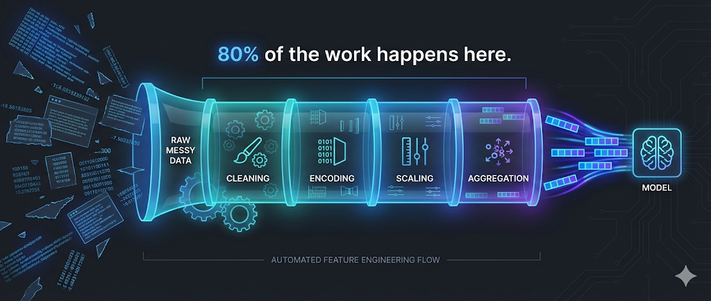
Key Insight: 80% of the work in machine learning isn’t choosing algorithms or tuning hyperparameters—it’s preparing and transforming data into useful features.

In automation, we know this intuitively:

• Writing a good Terraform module isn’t just about resource blocks
• It’s about input validation, variable transformation, conditional logic, and computed values
• The infrastructure code is 20%; the variable design and data flow is 80%

Feature engineering is the ML equivalent: transforming raw data into inputs that help the model learn patterns effectively.

We touched on this in Chapter 2.1, but now we’ll dive deeper into the specific techniques that make or break real ML projects.

---

Why Feature Engineering Matters More Than Algorithms

I tested this with our deployment risk model:

Experiment 1: Simple features + Random Forest

• Features: files_changed, hour, day_of_week
• Accuracy: 72%

Experiment 2: Engineered features + Decision Tree

• Features: is_large_change, is_business_hours, recent_failure_rate, team_reliability_score
• Accuracy: 86%

The takeaway: Better features with a simpler algorithm beat weak features with a complex algorithm.

Automation analogy:

• Good input validation + simple bash script > No validation + complex Python
• Well-structured Terraform variables + standard modules > Messy variables + custom code

---

The Feature Engineering Workflow

flowchart TD
    Start([Raw Data])
    
    Understand[1. Understand<br/>the Problem]
    Explore[2. Explore<br/>Raw Data]
    Create[3. Create<br/>New Features]
    Select[4. Select<br/>Best Features]
    Validate[5. Validate<br/>Impact]
    
    Model{Model<br/>Performance<br/>Good?}
    
    Deploy[Deploy to<br/>Production]
    Iterate[Iterate:<br/>New Ideas]
    
    Start --> Understand
    Understand --> Explore
    Explore --> Create
    Create --> Select
    Select --> Validate
    Validate --> Model
    
    Model -->|Yes| Deploy
    Model -->|No| Iterate
    Iterate --> Create
    
    style Start fill:#e3f2fd,stroke:#1976d2,stroke-width:2px
    style Deploy fill:#e8f5e9,stroke:#388e3c,stroke-width:3px
    style Model fill:#fff3e0,stroke:#f57c00,stroke-width:2px
    style Iterate fill:#ffebee,stroke:#d32f2f,stroke-width:2px

This looks like:

• Terraform development: Plan → Apply → Validate → Refactor
• CI/CD pipeline tuning: Build → Test → Analyze → Optimize

---

Technique 1: Encoding Categorical Variables

The Problem

ML algorithms work with numbers, not categories. But much of our data is categorical:

• Environment: dev, staging, prod
• Team: Platform, API, Frontend
• Deployment type: hotfix, feature, rollback

Solution: One-Hot Encoding

Automation analogy: Converting string variables into boolean flags.

# Terraform-style thinking
variable "environment" {
  type = string
  validation {
    condition = contains(["dev", "staging", "prod"], var.environment)
  }
}

locals {
  is_dev     = var.environment == "dev"
  is_staging = var.environment == "staging"
  is_prod    = var.environment == "prod"
}

ML implementation:

Original	→	is_dev	is_staging	is_prod
dev	→	1	0	0
staging	→	0	1	0
prod	→	0	0	1

When to Use

• Use one-hot encoding when:
  • Categories have no inherent order (dev isn’t “less than” prod)
  • You have fewer than 10-15 categories
• Alternatives for many categories:
  • Target encoding: Replace category with average outcome
  • Embedding: Let the model learn category representations (deep learning)

Example: Deployment Risk

Raw feature:
- deployment_type: "hotfix"

One-hot encoded:
- is_hotfix: 1
- is_feature: 0
- is_rollback: 0


> **Why this helps:** The model learns: hotfix → higher risk. Without encoding, "hotfix" is just a string (meaningless to the algorithm).
{: .prompt-tip }

---

Technique 2: Feature Scaling and Normalization

The Problem

Features with different scales can dominate the model:

Deployment	files_changed	duration_minutes	team_size
1	500	15	8
2	50	120	12

Issue: files_changed (0-1000) dominates team_size (5-20)

Solution: Normalize to Similar Scales

Automation analogy: Converting resource counts to percentages of capacity.

# Like monitoring thresholds
cpu_usage_percent = (current_cpu / max_cpu) * 100
memory_usage_percent = (current_memory / max_memory) * 100

# Both now on 0-100 scale, comparable

Common Scaling Methods

1. Min-Max Scaling (0 to 1)

scaled_value = (value - min) / (max - min)

Example:
files_changed: 500 → (500 - 0) / (1000 - 0) = 0.5
duration: 120 → (120 - 5) / (300 - 5) = 0.39

2. Standardization (Z-score)

scaled_value = (value - mean) / standard_deviation

Example:
files_changed: 500 → (500 - 200) / 150 = 2.0
(500 is 2 standard deviations above mean)

When to Use

• Min-Max: When you need values in a specific range (0-1, 0-100)
• Standardization: When you want to preserve outlier information
• No scaling: For tree-based models (Decision Trees, Random Forest) - they don’t care about scale

---

Technique 3: Binning and Discretization

The Problem

Sometimes continuous numbers are too granular. Grouping them into ranges can reveal patterns.

Solution: Create Bins (Buckets)

Automation analogy: Like alert severity levels.

# Monitoring thresholds
if cpu < 70:
    severity = "normal"
elif cpu < 85:
    severity = "warning"
else:
    severity = "critical"

ML application:

files_changed	→	change_size_category
5	→	small
50	→	medium
500	→	large

Binning Strategies

1. Equal-Width Bins

Small: 0-100 files
Medium: 101-500 files
Large: 501+ files

2. Equal-Frequency Bins (Quantiles)

Small: Bottom 33% of values
Medium: Middle 33%
Large: Top 33%

3. Domain-Driven Bins

Based on your expertise:
Small: 0-50 (safe deployments)
Medium: 51-200 (review required)
Large: 201+ (high risk)

When to Use

• Use binning when:
  • You have domain knowledge about meaningful thresholds
  • The relationship is step-wise, not smooth
  • You want interpretable categories
• Example: Deployment hour → is_business_hours is more useful than raw hour (14 vs 2)

---

Technique 4: Creating Interaction Features

The Problem

Sometimes the combination of features matters more than individual features.

The Insight

In automation, we know this:

# Terraform: Risk isn't just one variable
locals {
  high_risk = (
    var.environment == "prod" &&
    var.change_size == "large" &&
    var.time_window == "business_hours"
  )
}

ML equivalent: Create features that capture these interactions.

Example: Deployment Risk

Individual features:

• is_prod: 1
• is_large_change: 1
• is_business_hours: 1

Interaction feature:

• prod_AND_large_AND_business_hours: 1

Why this helps: The model learns “this specific combination is risky” more easily.

Common Interactions

flowchart LR
    F1[Feature 1:<br/>Environment]
    F2[Feature 2:<br/>Change Size]
    F3[Feature 3:<br/>Time]
    
    I1[Interaction:<br/>env_size]
    I2[Interaction:<br/>env_time]
    I3[Interaction:<br/>size_time]
    I4[Interaction:<br/>env_size_time]
    
    F1 --> I1
    F2 --> I1
    
    F1 --> I2
    F3 --> I2
    
    F2 --> I3
    F3 --> I3
    
    F1 --> I4
    F2 --> I4
    F3 --> I4
    
    style F1 fill:#e3f2fd,stroke:#1976d2,stroke-width:2px
    style F2 fill:#e3f2fd,stroke:#1976d2,stroke-width:2px
    style F3 fill:#e3f2fd,stroke:#1976d2,stroke-width:2px
    style I4 fill:#e8f5e9,stroke:#388e3c,stroke-width:3px

When to Use

• Use interaction features when:
  • Domain knowledge suggests combinations matter
  • Individual features alone don’t predict well
  • You have tree-based models (they can learn interactions, but explicit features help)
• Avoid when:
  • You have too many features (combinatorial explosion)
  • Using neural networks (they learn interactions automatically)

---

Technique 5: Time-Based Features

The Problem

Timestamps are hard for models to use directly: 2026-01-07 14:32:15 is just a number.

Solution: Extract Meaningful Time Components

Automation analogy: Parsing timestamps for scheduling logic.

# Like cron expressions or monitoring windows
from datetime import datetime

dt = datetime.now()
is_weekend = dt.weekday() >= 5
is_business_hours = 9 <= dt.hour < 17
is_end_of_month = dt.day > 25

Useful Time Features

From timestamp 2026-01-07 14:32:15:

Extracted Feature	Value	Why It Matters
hour	14	Deployment time affects risk
day_of_week	2 (Tuesday)	Weekday patterns
is_weekend	0	Weekend deployments riskier
is_business_hours	1	Business hours = more users affected
week_of_month	1	End of month rush?
is_end_of_sprint	1	Sprint deadlines = rushed deploys

Advanced: Lag and Rolling Features

Automation analogy: Like monitoring trends, not just current values.

Current deployment:
- current_cpu: 75%

Historical features:
- avg_cpu_last_7_days: 65%
- max_cpu_last_24h: 85%
- cpu_trend: increasing

These show context, not just snapshot

ML application:

Feature	Description	Example
deployments_last_7_days	Recent activity	12
failure_rate_last_30_days	Historical success	0.15
time_since_last_failure	Recency of issues	5 days
avg_duration_last_10	Typical duration	22 min

When to Use

• Use time features when:
  • Temporal patterns exist (time of day, day of week)
  • Historical context matters
  • Trends indicate risk (increasing failures, accelerating changes)

---

Technique 6: Aggregation and Summary Statistics

The Problem

Raw lists or sequences are hard to use: previous_deployments: [15, 22, 18, 30, 12]

Solution: Compute Summary Statistics

Automation analogy: Like log aggregation for metrics.

# Monitoring aggregation
response_times = [120, 135, 118, 450, 125]

metrics = {
    "avg": mean(response_times),      # 189.6
    "p95": percentile(response_times, 95),  # 450
    "max": max(response_times),       # 450
    "std_dev": std(response_times)    # High variance = inconsistent
}

ML application:

From [15, 22, 18, 30, 12] create:

• deployment_avg_duration: 19.4
• deployment_max_duration: 30
• deployment_std_dev: 6.8
• deployment_trend: increasing/decreasing

Common Aggregations

Metric	What It Captures
Mean	Typical value
Median	Central value (robust to outliers)
Max/Min	Extremes
Std Dev	Variability/consistency
Count	Frequency
Sum	Total

When to Use

• Use aggregations when:
  • You have historical sequences
  • Patterns exist in trends (not just current value)
  • Variability matters (consistent vs erratic behavior)

---

Feature Selection: Choosing What Matters

After creating features, you often have too many. Feature selection removes the noise.

Why Feature Selection Matters

Problems with too many features:

• ❌ Overfitting (model memorizes noise)
• ❌ Slower training
• ❌ Harder to interpret
• ❌ More storage and computation

Automation analogy:

• Too many Terraform variables = harder to use modules
• Too many monitoring metrics = alert fatigue
• Keep what adds value, remove the rest

Method 1: Correlation Analysis

Remove redundant features:

features_changed: 150
lines_changed: 3000

Correlation: 0.95 (highly correlated)
→ Keep one, drop the other

Method 2: Feature Importance (Tree-Based)

Let the model tell you what matters:

Random Forest feature importance:
1. recent_failure_rate: 0.35
2. is_prod: 0.25
3. change_size_category: 0.20
4. is_business_hours: 0.12
5. team_size: 0.08

→ Drop team_size (low importance)

Method 3: Recursive Feature Elimination

Iteratively remove least important features:

flowchart TD
    Start[Start with all features]
    Train1[Train model]
    Remove[Remove least important]
    Train2[Train again]
    Check{Performance<br/>still good?}
    Done[Final feature set]
    
    Start --> Train1
    Train1 --> Remove
    Remove --> Train2
    Train2 --> Check
    Check -->|Yes| Remove
    Check -->|No| Done
    
    style Start fill:#e3f2fd,stroke:#1976d2,stroke-width:2px
    style Done fill:#e8f5e9,stroke:#388e3c,stroke-width:3px
    style Check fill:#fff3e0,stroke:#f57c00,stroke-width:2px

Method 4: Domain Knowledge

Use your expertise:

Created features:
- deployment_size
- files_changed
- lines_added
- lines_deleted
- commit_message_length ← Probably useless
- author_name_length ← Definitely useless

→ Drop the obviously irrelevant ones

---

Practical Example: Deployment Risk (End-to-End)

Step 1: Start with Raw Data

deployment_id: 12345
timestamp: 2026-01-07 14:30:00
environment: prod
files_changed: 150
team: Platform
previous_deployments: [Success, Success, Failed, Success]

Step 2: Engineer Features

# Categorical encoding
is_prod = 1
is_staging = 0
is_dev = 0

# Binning
change_size = "large"  # (>100 files)

# Time features
hour = 14
is_business_hours = 1
day_of_week = 2
is_weekend = 0

# Historical aggregation
recent_failure_rate = 0.25  # (1/4 recent failures)
deployments_last_7_days = 8

# Interaction
prod_AND_large = 1  # (is_prod AND change_size=="large")

Step 3: Select Features

Feature importance ranking:
1. recent_failure_rate: 0.35
2. prod_AND_large: 0.28
3. is_business_hours: 0.18
4. deployments_last_7_days: 0.12
5. day_of_week: 0.07 ← Drop (low importance)

Final features: Top 4

Step 4: Result

Before feature engineering:

• Raw features: timestamp, environment, files_changed
• Accuracy: 72%

After feature engineering:

• Engineered features: recent_failure_rate, prod_AND_large, is_business_hours, deployments_last_7_days
• Accuracy: 88%

---

Feature Engineering Best Practices

1. Start Simple, Iterate

• ✅ Begin with obvious features
• ✅ Add complexity based on results
• ❌ Don’t create 100 features on day one

Automation analogy: Start with basic Terraform, refine based on needs.

---

2. Use Domain Knowledge

Your automation expertise is your superpower:

• You know peak hours matter → Create is_business_hours
• You know team reliability varies → Create team_success_rate
• You know change size indicates risk → Create change_size_category

This beats blindly trying transformations.

---

3. Validate Feature Impact

Test each feature:

Baseline (no feature): 75% accuracy

Add recent_failure_rate: 82% accuracy ✅ Keep it
Add commit_message_length: 75% accuracy ❌ Drop it
Add prod_AND_large: 85% accuracy ✅ Keep it

---

4. Avoid Data Leakage

Data leakage = Using information that won’t be available at prediction time

Bad example:

# Feature: deployment_duration
# Label: deployment_success

Problem: You don't know duration until AFTER deployment completes
→ Can't use this feature to predict success before deploying

Automation analogy: Can’t use the result to predict the result.

---

5. Document Your Features

Future you (and your team) will thank you:

features:
  recent_failure_rate:
    description: "Ratio of failed deployments in last 30 days"
    calculation: "failures / total_deployments (last 30 days)"
    range: "0.0 to 1.0"
    
  prod_AND_large:
    description: "High risk indicator: production + large change"
    calculation: "is_prod AND change_size=='large'"
    values: "0 or 1"

---

My Feature Engineering Checklist

Before building a model, I now ask:

1. What domain knowledge can I encode?
   • Time patterns, business rules, known thresholds
2. Are categorical variables encoded?
   • One-hot encoding, target encoding, or embeddings
3. Are scales normalized?
   • If using distance-based algorithms (KNN, SVM)
4. Have I created interaction features?
   • Combinations that matter based on expertise
5. Have I extracted time components?
   • Hour, day, business hours, trends
6. Have I aggregated historical data?
   • Means, trends, failure rates
7. Have I tested feature importance?
   • Drop low-value features
8. Am I avoiding data leakage?
   • Only use information available at prediction time

---

Key Takeaways

Key Takeaways:

• Feature engineering is 80% of ML work: Good features + simple algorithm > Bad features + complex algorithm
• Your domain expertise is your biggest advantage
• Common techniques:
  • One-hot encoding: Convert categories to numbers
  • Scaling: Normalize feature ranges
  • Binning: Group continuous values into categories
  • Interactions: Combine features that matter together
  • Time features: Extract meaningful time components
  • Aggregations: Summarize historical patterns
• Feature selection matters: Remove redundant features, use feature importance rankings, keep what adds value, drop the rest
• Think like an automation engineer: Feature engineering = data transformation pipelines (like Terraform locals, Ansible filters, data preprocessing). Apply the same rigor you apply to infrastructure code.

---

What’s Next?

➡ Series 4 – Deep Learning

In the next series, we’ll explore:

• Why deep learning exists
• How neural networks work (without the math)
• When to use deep learning vs traditional ML
• The connection to LLMs and generative AI

Architectural Question: How does deep learning change the role of feature engineering, and when should you trust a neural network to learn features for you?

The key insight: Deep learning automates feature engineering—the network learns features from raw data instead of you manually creating them.

---